|
|
Last Update: April 8,
2011
|
|
|
|
Table of contents
1.Power Series Solutions
2
1.1.Why is a power series sometimes referred
to as “formal”? 2
1.2.Why is the “radius of
convergence” the distance from  to
its closest complex singular point?
2
to
its closest complex singular point?
2
1.3.Is the radius of convergence useful in
practice? 3
2.Fourier Series and Related
3
2.1.What is an eigenvalue problem? What is an
eigenvalue? 3
2.2.Why are eigenvalues that are larger than
zero insignificant? 4
2.3.In the case  , how
would you ever get an eigenvalue? Your general solution does not
even have a
, how
would you ever get an eigenvalue? Your general solution does not
even have a  ! 4
! 4
2.4.Why do we discuss three cases  ? 4
? 4
2.5.Why is there generally still a constant in
the eigenfunction? Will this always be the case?
5
2.6.When solving the eigenvalue problems, why
do we sometimes write  instead of
  ? 5
? 5
2.7.Why is the factor  for Fourier cosine and Fourier sine, but
  for Fourier? 5
2.8.Why is the constant term written as  in Fourier and Fourier cosine series? 5
2.9.Are Fourier cosine and Fourier sine series
special cases of Fourier series? 6
3.Separation of Variables
7
3.1.How do I know when it's Fourier Cosine and
when it's Fourier Sine? 7
1.Power Series Solutions
1.1.Why is a power series sometimes referred
to as “formal”?
Ans.
A power series is a combination of numbers  , and a symbol
  in the following
particular manner:
in the following
particular manner:

or equivalently  .
.
Such an infinite sum is often called “formal” because
-
At this stage, without assigning any value to ,
it is just a particular way of writing the numbers ,
and the symbol
together, nothing more. In particular it does not represent anything
such as a “function of ”.
-
Even if we assign some value to , say let
 , the resulting infinite sum of numbers

still may or may not converge. When it converges, it represents a
number; When it does not, it represents nothing.
In summary, a power series represents a function
only inside some interval  . Outside, the meaning
of is not clear and is thus purely formal (Many
researchers have been trying to give meaning to the sum for outside the convergence disk. Such research results in
many “named sums”: Cesaro sum, Borel sum, etc. )
. Outside, the meaning
of is not clear and is thus purely formal (Many
researchers have been trying to give meaning to the sum for outside the convergence disk. Such research results in
many “named sums”: Cesaro sum, Borel sum, etc. )
1.2.Why is the “radius of
convergence” the distance from to its
closest complex singular point?
Ans.
First the distance from to its closest complex
singular point is just a lower bound of the radius of convergence of the
power series solution – meaning the radius is at least as large.
A full understanding of the “why” involves tedious
calculation which can fill a couple of pages. But quick
“pseudo-understanding” may be achieved through the
following.
Consider a power series  which solves a linear
differential equation whose singular points are
which solves a linear
differential equation whose singular points are  ,.
,.
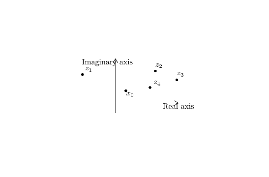 |
|
Figure 1. (Hypothetical) distribution of
singular points
|
First, it is crucial to think of the in a power
series not as only a real number, but a complex number. Thus for any
complex number  , we can set
  in the formal power series and obtain an infinite sum of numbers:
Next, the fact is that, for each value
, this infinite sum either converges or does not converge. It turns out
that, for all
such that
 , the sum converges, while for all
such that
, the sum converges, while for all
such that
 , the sum diverges. As a consequence, all the
's in the complex plane with the sum converges form a disk centered at
with radius
, the sum diverges. As a consequence, all the
's in the complex plane with the sum converges form a disk centered at
with radius
 – hence the name “radius of convergence” (If we only
consider the real line, “distance of convergence” would be a
better name!).
– hence the name “radius of convergence” (If we only
consider the real line, “distance of convergence” would be a
better name!).
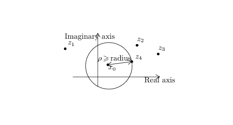
It turns out that, this converging disk can be at least so large that no
singular point is inside it. Therefore the best we can do is to
“expand” this disk until its boundary “touches”
a singular point:
 |
|
Figure 2. Largest disk we can have without
including any singular point.
|
1.3.Is the radius of convergence useful in
practice?
Ans.
Indeed it is. For example, suppose after some great effort we have found
out the first 4 terms of a power series solution

and have concluded that it is not possible to write down a general
formula for the generic coefficient  .
.
Thus we have to get some idea of  using the first
4 terms. Naïvely we expect is close to
using the first
4 terms. Naïvely we expect is close to  . But how confident are we? Do we have any idea for
which this is true and for which this is not? We have no idea.
. But how confident are we? Do we have any idea for
which this is true and for which this is not? We have no idea.
Things change when we have the extra information of radius of
convergence. Say we found out that  . Now we can
conclude:
. Now we can
conclude:
-
For
 , it's not a good idea to use to approximate ;
-
For
 , such approximation is possible.
Furthermore the smaller
, such approximation is possible.
Furthermore the smaller  is, the better the
approximation.
is, the better the
approximation.
2.Fourier Series and Related
2.1.What is an eigenvalue problem? What is an
eigenvalue?
Ans.
An “eigenvalue problem” is a linear, homogeneous boundary
value problem involving one unknown number. For example

is an eigenvalue problem. So an “eigenvalue problem” is in
fact a collection of infinitely many boundary value
problems.
If we assign a number to , the eigenvalue problem
“collapses” to a usual boundary value problem. For example,
if we set  , the above problem
“collapses” to
, the above problem
“collapses” to

As an “eigenvalue problem” is linear and homogeneous,  is always a solution, no matter what number is assigned. On the other hand, there usually exist a
bunch of special numbers such that, when assigned to ,
the resulting boundary value problem has (besides )
non-zero solutions. These “special numbers” are called
“eigenvalues”.
is always a solution, no matter what number is assigned. On the other hand, there usually exist a
bunch of special numbers such that, when assigned to ,
the resulting boundary value problem has (besides )
non-zero solutions. These “special numbers” are called
“eigenvalues”.
For example, consider the eigenvalue problem:

We try:
-
. The problem becomes
 .
Solving it, we see that the only solution is .
So
.
Solving it, we see that the only solution is .
So  is not an eigenvalue for the problem.
-
 . The problem becomes
  which has, besides , at least one non-zero
solution
which has, besides , at least one non-zero
solution  (as well as
  and in fact
  for arbitrary number
  ). Therefore
  is an eigenvalue for
the problem.
is an eigenvalue for
the problem.
A word of caution here: An eigenvalue problem consists of three parts:
an equation (involving ) and two boundary
conditions. Slight change to any one part of the three may lead to
big change in the looks of eigenvalues/eigenfunctions as well as the
range of  !
!
2.2.Why are eigenvalues that are larger than
zero insignificant?
Ans.
They are not insignificant. All eigenvalues are
significant, larger than zero or not. Following N. Trefethen, we can say
the set of all eigenvalues is the “signature” of the
differential equation. We only see non-positive eigenvalues in class
because we have only solved a couple of the simplest eigenvalue
problems. It's purely accidental that there is no positive eigenvalue
for these problems. If we have chance to see more sophsticated ones,
there will be eigenvalues of both signs.
It should be emphasized that the question itself is not
correct. For the eigenvalue problems we dealt in
class, any  cannot be an eigenvalue. So it's not
that “eigenvalues ... larger than zero insignificant”, but
“no eigenvalues larger than zero at all”.
cannot be an eigenvalue. So it's not
that “eigenvalues ... larger than zero insignificant”, but
“no eigenvalues larger than zero at all”.
2.3.In the case , how
would you ever get an eigenvalue? Your general solution does not even have
a !
Ans.
Recall that an eigenvalue is just a number such that, if is set to this number, the resulting boundary value
problem has non-zero solutions. So the whole discussion of the case is just checking whether is
an eigenvalue or not: If we set in the problem,
does the resulting boundary value problem have any non-zero solution? If
the answer is yes, then is an eigenvalue; If the
answer is no, then is not an eigenvalue.
For example, consider the eigenvalue problem
If we set , the problem becomes  which gives as the only solution. So is not an eigenvalue for this problem.
On the other hand, if we consider a different eigenvalue problem

Setting gives  which
indeed has non-zero solutions, for example
which
indeed has non-zero solutions, for example  . So
is an eigenvalue for this problem.
. So
is an eigenvalue for this problem.
2.4.Why do we discuss three cases ?
Ans.
First it should be emphasized that this only happens when the equation
in our problems if  . If we change the equation,
the cases will be different.
. If we change the equation,
the cases will be different.
To understand why, we track how we find eigenvalues.
-
The basic idea of finding eigenvalues is to try every number: Assign
it to and see whether any non-zero solution
exists;
-
Naïve implementation of this strategy clearly would not work.
Instead, we observe that, for the problem with equation , all possible values of can be
categorized into three cases:
 . In each case,
we can write down a formula for the solution
. In each case,
we can write down a formula for the solution  which is true for all in that case. For
example, no matter what number we assign to ,
as long as it's positive, must take the form
which is true for all in that case. For
example, no matter what number we assign to ,
as long as it's positive, must take the form
 .
.
2.5.Why is there generally still a constant in
the eigenfunction? Will this always be the case?
Ans.
Yes this will always be the case. There will always be arbitrary
constants in the formulas for eigenfunctions, and the number of such
constants can be any positive number: one, two, three...
To understand why, we take a look at the eigenvalue problems we have
solved:


in the last one  are the roots of the
transcendental equation
are the roots of the
transcendental equation  . Also notice that in the
3rd problem two arbitrary constants are involved in the formula of the
eigenfunction.
. Also notice that in the
3rd problem two arbitrary constants are involved in the formula of the
eigenfunction.
All these problems are linear and homogeneous, which means if
 solves the problem, so is
  ,
where
,
where  are arbitrary constants. This property is
enjoyed by all eigenvalue problems. As a consequence, if there is any
nonzero solution to the problem, then automatically its constant
multiples are also solutions.
are arbitrary constants. This property is
enjoyed by all eigenvalue problems. As a consequence, if there is any
nonzero solution to the problem, then automatically its constant
multiples are also solutions.
2.6.When solving the eigenvalue problems, why
do we sometimes write instead of ?
Ans.
The reason is we would like to write every complex number in its
standard form  where
where  are
real. For example, if we have
are
real. For example, if we have  , we usually write
it as
, we usually write
it as  instead of just .
So when , we just write
as this is a real number; But when  , we prefer
writing
, we prefer
writing  over because the
latter is not in “standard form”.
over because the
latter is not in “standard form”.
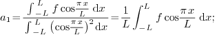
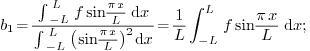
2.7.Why is the factor
for Fourier cosine and Fourier sine, but for
Fourier?
Ans. The reason lies in that all three are special
cases of orthogonal systems.  and
and  are orthogonal systems with weight
  over the interval
  , while
 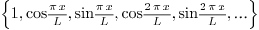 is an orthogonal system with weight over the
interval
is an orthogonal system with weight over the
interval  (note the interval is different!).
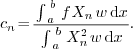
If  is an orthogonal system over
  with weight
  , then the coefficients of the
expansion
, then the coefficients of the
expansion

can be found through
Now we have

which explains the different factors.
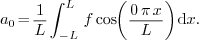
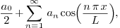
2.8.Why is the constant term written as in Fourier and Fourier cosine series?
Ans.
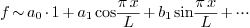
Consider the Fourier series, where any  is
expanded with respect to the orthogonal system
is
expanded with respect to the orthogonal system 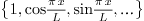 (which is orthogonal over with weight
  ). From the theory of orthogonal systems, we know that if
we write
). From the theory of orthogonal systems, we know that if
we write
then the coefficients are given by
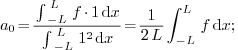
and so on. We see that the formulas for all
except  can be written as
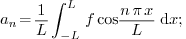
This is not beautiful. To make things look better, instead of 
 we write
  so that the new is the same
as two times the old one, and can be computed through
so that the new is the same
as two times the old one, and can be computed through
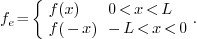
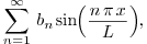
2.9.Are Fourier cosine and Fourier sine series
special cases of Fourier series?
Ans. No.
-
On the theoretical side, all three (Fourier cosine, Fourier sine and
Fourier) are special cases of orthogonal systems arising from
solving eigenvalue problems.
-
 gives Fourier;
-
 gives Fourier sine;
-
 gives Fourier cosine.
No one is at a higher level or “more general” than
another.
-
On the other hand, on the practical side, one can obtain the
coefficients in a Fourier cosine or Fourier sine expansion of a
certain function by computing the
coefficients of the Fourier expansion of another
function which is related to through:
Such properties can be used to analyze the convergence properties of
the Fourier cosine and Fourier sine expansions (although such detour
becomes obsolete once one learns the full Sturm-Liouville theory).
3.Separation of Variables
3.1.How do I know when it's Fourier Cosine and
when it's Fourier Sine?
Ans.
The short answer is, you know automatically from solving the eigenvalue
problem. If after solving the eigenvalue problem, you get  for certain
  (usually given in the problem in the form – it can be given in other forms), then the initial
value should be expanded into Fourier cosine series; If you get
(usually given in the problem in the form – it can be given in other forms), then the initial
value should be expanded into Fourier cosine series; If you get  , Fourier sine.
The above guarantees quick reaction in exams. But a quiet mind and
fearless heart can be reached through understanding the reason behind
this mess. The fundamental reason is the following:
 's turn out to be the same as
those
's turn out to be the same as
those 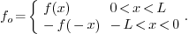
 form an orthogonal system
with certain weight
form an orthogonal system
with certain weight  , which means
 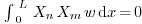 whenever
  . Consequently the
expansion of any function
. Consequently the
expansion of any function 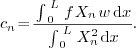
 .
.